Approximating Struve functions

As special functions go, it seems the Struve function goes somewhat unloved. Whilst one cannot move for implementations of Bessel function, both the default MATLAB package and the Julia programming language are left lacking, leaving the programmer to roll their own.

Sadly, the usual trick of heading over to Wikipedia to look an easy approximation doesn’t end with easy answers. Likewise, whilst Zhang and Jin has a chapter on Struve functions, it doesn’t go beyond the power series expansion found in Abramowitz and Stegan.

This left me a little lost. Olver et al. suggest the direct evaluation of power series, but don’t give guidance on the number of terms or when to switch to the large z expansion. Other authors present their approximations, but don’t delve extensively into the error of their approximation. Here, I aim to explore this a little.

A little about Struve functions

Struve functions are a component of a general solution to a nasty differential equation. However, for me they showed up in integral form. As a special function, there is no neat means by which to evaluate them. The Struve functions are \(\mathbf{H}_v(z)\) and \(\mathbf{K}_v(z)\), and the modified Struve functions are \(\mathbf{L}_v(z)\) and \(\mathbf{M}_v(z)\). \(\mathbf{K}_v(z)\) and \(\mathbf{M}_v(z)\) can be obtained from \(\mathbf{H}_v(z)\) and \(\mathbf{L}_v(z)\) through the subtraction of Bessel functions and modified Bessel functions. Since approximations of Bessel functions are everywhere, I consider this a non-issue. Likewise, the Struve function \(\mathbf{H}_v(z)\) is related to the modified Struve function \(\mathbf{L}_v(z)\) by the formula

meaning that so long as Struve function \(\mathbf{H}_v(iz)\) can be evaluated, we can obtain every other variety.

Furthermore, recurrence relations can be used to obtain Struve functions of any integer order given \(\mathbf{H}_0(z)\) and \(\mathbf{H}_1(z)\).

Consequently, this post focuses on \(\mathbf{H}_0(z)\) and \(\mathbf{H}_1(z)\), seemingly the most studied orders. I won’t consider non-integer orders.

Power series expansion

Looking in Abramowitz and Stegan (or Olver et al.) will give you a definition of the Struve function \(\mathbf{H}_v(z)\). However, I’ll jump straight to the most obvious method of evaluation - the power series expansion:

and for \(v=0\) and \(v=1\)

These series are easy to program and always convergent. Care must be taken to using floating point in the denominator - an integer will rapidly overflow.

A large number of terms are required to achieve good accuracy. To obtain a solution with a relative error of approximately 1e-6, the number of terms required in the \(\mathbf{H}_0(z)\) expansion are plotted:

And for \(\mathbf{H}_1(z)\):

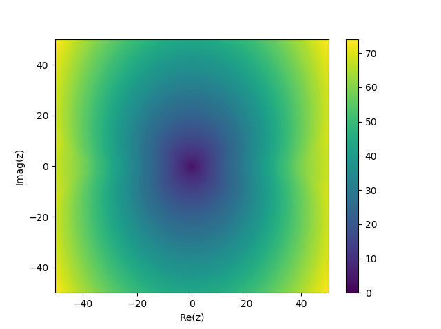
The number of terms required gets bigger scales with \(\vert z \vert\).

For large values of \(z\) Abramowitz and Stegan give asymptotic expansions:

The numerator in each term of these expansions grows faster than the denominator, to my mind implying infinite truncation error for any finite argument. None the less, taking the just the first term of these and combining with the large value expansion \(Y_v(z) = \sqrt{2 / (\pi z)}\sin(z - \pi v / 2- \pi / 4)\) (A&S 9.2.2) gives:

Naturally, its unclear what constitutes large \(z\). I therefore compared these approximations to the Python mpmath implementation using 25 digits of precisions for real x. The relative accuracy of these approximations was disappointing:

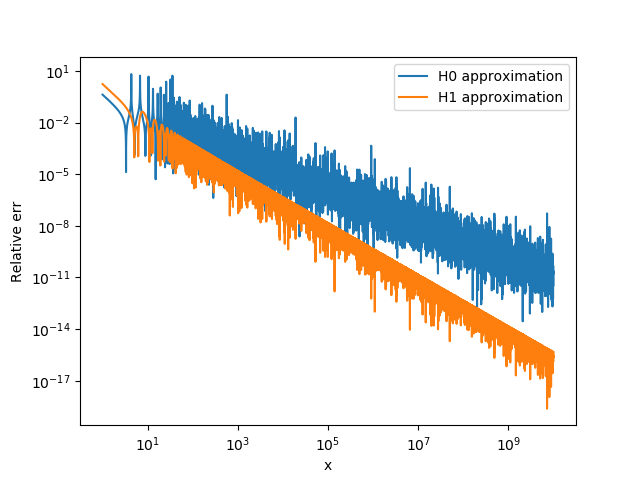
The main source of error here appears to be the Bessel function approximation. Using instead

Additionally we can add additional terms to the expansion. The results for real x are show:

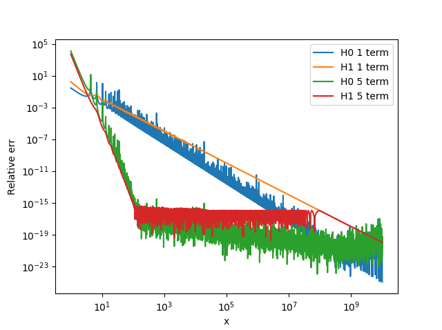
Certainly the approximation of the Bessel function results in significant errors. Presumably the noise in the \(\mathbf{H}_0(x)\) 1 term curve and the 5 term curves is due to the introduction of double precision numbers into the calculations. The addition of multiple terms is also very beneficial. The implications of computing the approximation in double precision is noticeable.

A composite of the two methods can be used. If a 60 term power series is used for \(\vert z \vert < 20\) and the large value expansion with 7 terms is used otherwise, the following results are obtained for \(\mathbf{H}_0(z)\):

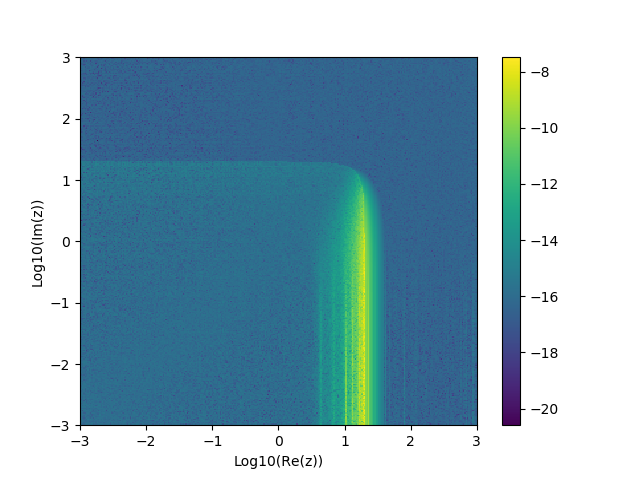
And for \(\mathbf{H}_1(z)\):

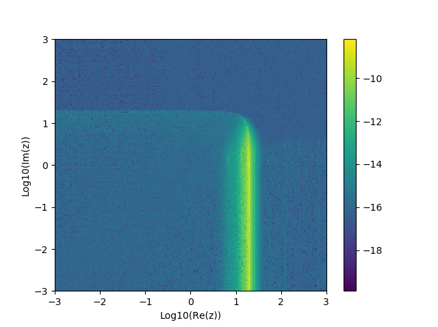
Reasonable results can be obtained. However, for large portions of the domain, the computational cost could be reduced significantly by changing the number of terms. The most difficult region seems to be when the real part is around 20. Accuracy is only single precision despite the computational effort.

Aarts and Janssen’s approximations

Aarts & Janssen develop an approximation as follows:

The log10 of the relative error can be plotted.

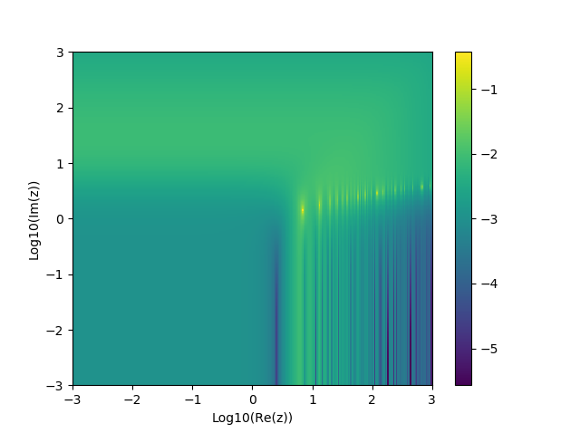
and \(\mathbf{H}_0(z)\) as

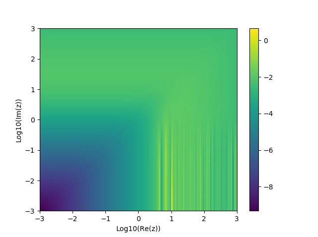
Evidently, whilst these expressions are convenient, they leave something to be desired with respect to accuracy.

Piecewise polynomial approximation

Newman describes a composite approach for real \(x\).

For real \(x\) where \(0 \leq x \leq 3\):

where \(\vert \epsilon_0 \vert < 1.2 \times 10^{-8}\) and \(\vert \epsilon_1 \vert < 2.5 \times 10^{-9}\).

For real \(x\) where \(x \geq 3\):

where \(\vert \epsilon_0 \vert < 8.2 \times 10^{-9}\) and \(\vert \epsilon_1 \vert < 2.5 \times 10^{-8}\).

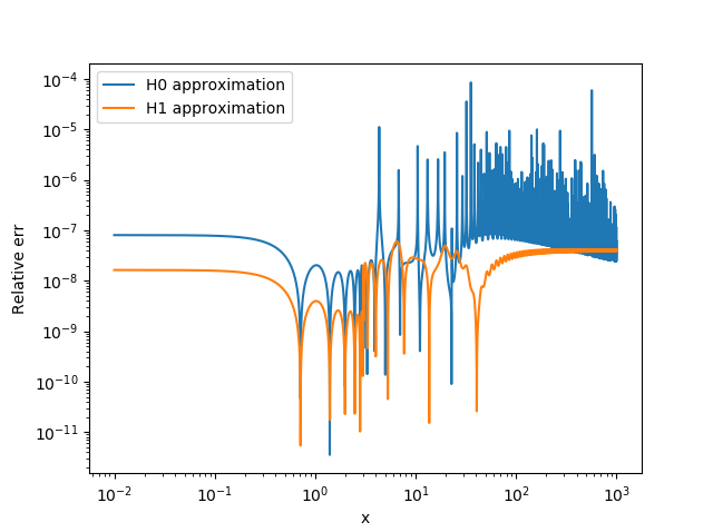
Plotting the absolute error suggests that the error estimations are not overstated, even with the small number of terms used in the approximations:

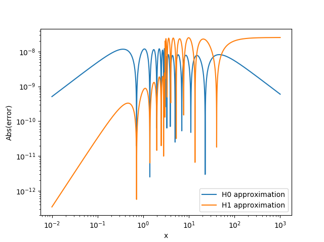
Although in some places the relative error is somewhat higher than can be achieved using the asymptotic expansion for large values of z:

Via Quadrature

Struve functions have integral forms. We can directly obtain approximations using quadrature therefore. This is something I’m reluctant to delve into however - the integrands are oscillatory.

How are other people actually doing it?

As wonderful as consulting outdated papers is, a pragmatic approach would be to follow the others of others. I found several implementations:

• Python: SciPy: A mixed approach. Large z expansion if \(z \geq 0.7v + 12\), expansion in Bessel functions if \(\vert z \vert < \vert v \vert + 20\). A power series otherwise.
• Python: mpmath: Using hypergeometric series (power series). I think.
• MATLAB: (Struve function on File Exchange): Chebyshev expansions for small z, and rational approximations for large z - much like a higher accuracy version of Newman.
• C: CEPHES: Hypergeometric series (power series).

Conclusions (for now)

There appears to be no easy, accurate approximation for the Struve functions. To me, the most promising approach seems to be Chebyshev expansions, as used in the MATLAB implementation and Newman. These require effort to produce. A quick implementation probably does best to directly evaluate the power series. This has been my path forward.

References

• Frank W.J. Olver, Daniel W. Lozier, Ronald F. Boisvert and Charles W. Clark, NIST Handbook of Mathematical Functions Paperback and CD-ROM, Cambridge University Press, 2010

• M. Abramowitz and I. Stegun, Handbook of Mathematical Functions with Formulas, Graphs, and Mathematical Tables, United States Department of Commerce, National Bureau of Standards, 1964

• Ronald M. Aarts and Augustus J. E. M. Janssen, Approximation of the Struve function H1 occurring in impedance calculations, Acoustical Society of America, 2003.

• Ronald M. Aarts and Augustus J. E. M. Janssen, Efficient approximation of the Struve functions Hn occurring in the calculation of sound radiation quantities, 2016.

• J. N. Newman, Approximations for the Bessel and Struve Functions, Mathematics of Computation, 1984

• R. Zanovello, Sul calcolo numerico della funzione di Struve Hv⁢ (z), Rend. Sem. Mat. Univ. e Politec. Torino, 1975.

Hugh Bird

A Post-graduate research student at the University of Glasgow, United Kingdom.

About